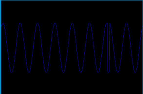
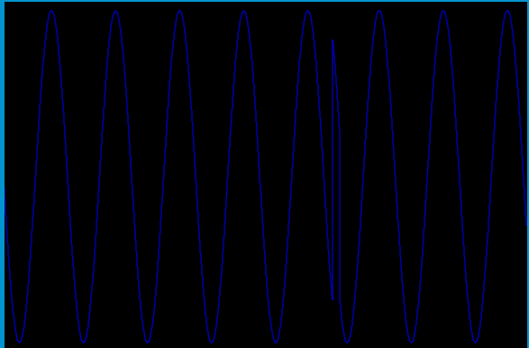
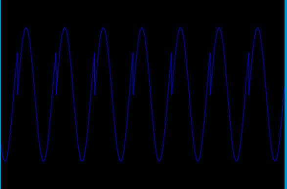
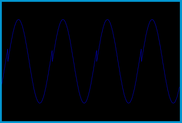
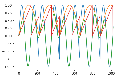
I have created a “test-tube” with python and ctcsound in order to visualize your HardSyncOscillator example. I really try to understand the importance of the envelope. (As if you are trying to eliminate clicks…) Anyway, I am encouraged to use the technique myself, as it works in ksmps = 32.
These are the first 1024 audio samples. 32 cycles times 32 samples per cycle (ksmps=32).
a2 = blue, aEnv = yellow, aout = green, and phase2 = red
More interesting is the python code I wrote. Could be useful to anyone.
import ctcsound
import numpy as np
from matplotlib import pyplot as plt

ach1 = []
ach2 = []
ach3 = []
aph  = []

orc_text = '''
 ksmps = 32
 nchnls = 2
 0dbfs = 1

 giHalfSine ftgen 0,0,4097,9,0.5,1,0
 instr 1
    kFreq1            chnget      "freq1"
    kFreq2            chnget      "freq2"
    aphase1,asyncout1 syncphasor  kFreq1, a(0)
    aphase2,asyncout2 syncphasor  kFreq2, asyncout1
    a1                tablei      aphase1, -1,1,0,1
    a2                tablei      aphase2,-1,1,0,1
    aEnv              tablei      aphase1,giHalfSine,1
    aout              =            a2 * aEnv
                      chnset      a2, "ch1"
                      chnset      aEnv, "ch2"
                      chnset      aout, "ch3"
                      chnset      aphase2, "cph"
                      outs        aout,aout
 endin
'''

sco_text = "i 1 0 5"

cs = ctcsound.Csound()
cs.setOption("-d")
cs.setOption("-odac")
cs.compileOrc(orc_text)
cs.readScore(sco_text)

cs.start()

cs.setControlChannel("freq1", 200)
cs.setControlChannel("freq2", 330)

i=0

while cs.performKsmps()==False and i<32:
    atemp1 = cs.channelPtr("ch1", ctcsound.CSOUND_AUDIO_CHANNEL)
    ach1 = np.append(ach1, atemp1[0])
    atemp2 = cs.channelPtr("ch2", ctcsound.CSOUND_AUDIO_CHANNEL)
    ach2 = np.append(ach2, atemp2[0])
    atemp3 = cs.channelPtr("ch3", ctcsound.CSOUND_AUDIO_CHANNEL)
    ach3 = np.append(ach3, atemp3[0])
    atemp4 = cs.channelPtr("cph", ctcsound.CSOUND_AUDIO_CHANNEL)
    aph = np.append(aph, atemp4[0])
    i += 1

fig, ax = plt.subplots()
ax.plot(ach1)
ax.plot(ach2)
ax.plot(ach3)
ax.plot(aph)

cs.cleanup()
cs.reset()
del cs


